- Published on
HPCG: 3. Sparse Matrix Formats and Memory Access Optimization
- Authors
- Name
- Han, Minhee
TL;DR
The reference HPCG implementation uses the Compressed Sparse Row (CSR) format for representing sparse matrices. The ELLPACK format can provide better memory access patterns for the computation. In addition, by reordering(permuting) rows and elements in matrices and vectors, we can further optimize the memory access pattern.
Sparse Matrix Formats
One major characteristics of matrices in HPCG is that they are sparse, (with lots of 0 values) and thus, how we represent these matrices can affect the performance of the computation. There are several formats to represent sparse matrices, and each has its own characteristics. In this article, we will look at the COO (Coordinate List), CSR (Compressed Sparse Row), and ELLPACK formats.
Dense Matrix
It's the matrix format we know of. Let's say we have a matrix like this:
dense_matrix_1 = np.array([
    [10, 0, 0, 0, 0],
    [0, 20, 0, 0, 0],
    [30, 0, 0, 0, 40],
    [0, 0, 0, 50, 0],
    [0, 0, 0, 0, 0]
])
We can see that most of the elements are zero. It's clear that we can save a lot of memory by not storing these zero elements. This is where sparse matrix formats come in.
COO (Coordinate List)

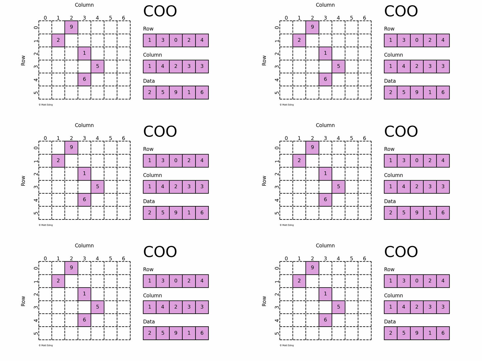
In the COO format, we store the non-zero elements along with their row and column indices. For the above matrix, we can get the COO format like this:
def dense_to_coo(matrix):
    data = matrix[matrix != 0]  # Non-zero values
    row, col = np.nonzero(matrix)  # Indices of non-zero values
    return row, col, data
the resulting coo format will be like this:
row, col, data  = dense_to_coo(dense_matrix_1)
print(row)
# [0 1 2 2 3]
print(col)
# [0 1 0 4 3]
print(data)
# [10 20 30 40 50]
The first non-zero value is 10, and it's located at [0,0]. Thus we save 10, 0, 0 to the data, row, and col arrays respectively. We repeat this for all non-zero values. 40 is at [2,4], so we save 40, 2, 4 to the arrays.
This format is easy to implement and simple, but it requires accessing three arrays for a single value. Also, to find a given row, as we need to find all row indices corresponding row and then we can find the column indices, it can be inefficient.
CSR (Compressed Sparse Row)

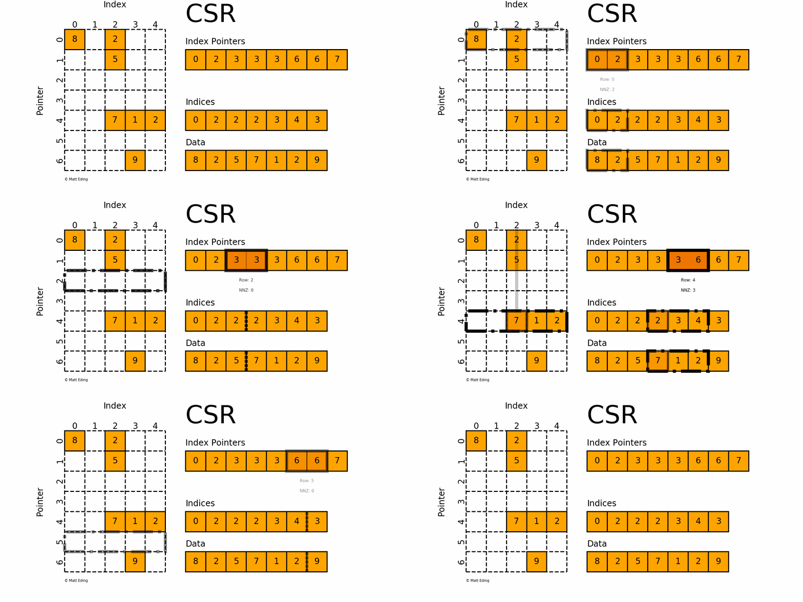
This is used as the default format in the HPCG benchmark. As its name suggests, the CSR format compresses the COO format by storing not the row index for each value, but the pointers to the column index array where each row begins. For the above matrix, the CSR format would look like this:
def dense_to_csr(matrix):
    data = matrix[matrix != 0]  # Non-zero values
    row, col = np.nonzero(matrix)  # Indices of non-zero values
    row_ptr = np.zeros(matrix.shape[0] + 1, dtype=int)
    for r in row:
        row_ptr[r + 1] += 1
    row_ptr = np.cumsum(row_ptr)
    return row_ptr, col, data
row_ptr, col, data = dense_to_csr(dense_matrix_1)
print(row_ptr)
# [0 1 2 4 5 5]
print(col)
# [0 1 0 4 3]
print(data)
# [10 20 30 40 50]
row_ptr is an array that stores the starting index of each row in the col and data arrays. The second element 1 means that the column and data index for the second row starts from 1. The third element 2 means that the column and data index for the third row starts from 2. Thus, there is only one element in the second row(2 - 1 = 1) and its column index is 1 (col[1]) and the data is 20 (data[1]). Likewise, the third and the fourth element in the row_ptr array are 2 and 4, which means that the third row has two elements. The column indices are cold[2:4] and the values are data[2:4]. The last two elements in the row_ptr array are 5, which means that the last row has zero element (5 - 5 = 0). We still need these indices to show how much rows are there in the matrix.
Compared to COO, CSR is more efficient in accessing a row, as it only needs two values in the row pointer array before getting column indices. However, it doesn't seem that "compressed" in this example. Consider this matrix:
dense_matrix_2 = np.array([
    [1, 2, 3],
    [4, 5, 6],
    [7, 8, 9]
])
"Compressed" Examples
#  print dense_matrix_2 in coo format
row, col, data = dense_to_coo(dense_matrix_2)
print(row)
# [0 0 0 1 1 1 2 2 2]
print(col)
# [0 1 2 0 1 2 0 1 2]
print(data)
# [1 2 3 4 5 6 7 8 9]
# print dense_matrix_2 in csr format
row_ptr, col, data = dense_to_csr(dense_matrix_2)
print(row_ptr)
# [0 3 6 9]
print(col)
# [0 1 2 0 1 2 0 1 2]
print(data)
# [1 2 3 4 5 6 7 8 9]
We can see that the CSR format is more efficient in this case. However, it isn't a good example as we're mostly dealing with sparse matrices. The examples are too small to demonstrate the characteristics of the formats. Thus, let's generate a large sparse matrix and see how the formats differ.
#  Generate a random sparse matrix 1024*1024 in naive dense format
dense_matrix_3 = np.random.rand(1024, 1024)
dense_matrix_3[dense_matrix_3 < 0.9] = 0 # 90% sparsity

#  print the space used by dense_matrix_3 in coo format
row, col, data = dense_to_coo(dense_matrix_3)
print(len(row) + len(col) + len(data))
# 315873

#  print the space used by dense_matrix_3 in csr format
row_ptr, col, data = dense_to_csr(dense_matrix_3)
print(len(row_ptr) + len(col) + len(data))
# 211607
We can see that the space needed for the CSR format is smaller than one for the COO format in this case. It is generally more efficient space-wise than COO format for large matrices.
inefficiency of CSR in Parallelization
However, the problem with CSR is that we cannot coalesce memory access. Regarding parallelization, we can make each thread to work on a row. When accessing a certain row, however, we cannot determine which part of the data array and the column index array each thread will access. Think of a matrix multiplcation for our matrix:
dense_matrix_4 = np.array([
    [10, 0, 0, 70, 0, 40],
    [0, 20, 0, 0, 0, 10],
    [30, 0, 0, 0, 40, 0],
    [0, 0, 0, 50, 0, 0],
    [0, 0, 70, 0, 60, 10],
    [0, 0, 0, 0, 0, 0]
])

row_ptr, col, data = dense_to_csr(dense_matrix_4)
print(row_ptr)
# [ 0  3  5  7  8 11 11]
print(col)
# [0 3 5 1 5 0 4 3 2 4 5]
print(data)
# [10 70 40 20 10 30 40 50 70 60 10]
thread 0 handles first row, and it needs data[0:3], thread 1 needs data[3:5]. So, when accessing the first element, thread 0 will access data[0] while thread 1 will access data[3]. Because of the irregularity of the location in the arrays, it's hard to find a way to coalesce the memory accesses. Imagine larger matrices and more threads. If we can coalesce 32 values at the same time, the number of nonzeros in a row larger than 32 will ruin memory coalescing among threads. Thus, we need to find a format that will enable adjacent threads to access adjacent memory locations, thus enabling memory coalescing.
ELLPACK

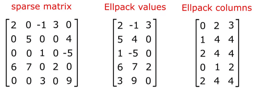
This is the recommended format for the HPCG benchmark. In ELLPACK, instead of saving row related indices, we just use fixed amount of memory for each row. In HPCG, the number of non-zero elements per row is fixed, up to 27, and thus we make ELLPACK format with 27 as the fixed width. ELLPACK is efficient for sparse matrices with small variants in numbers of non-zero elements per row.
- Set the ELLPACK width as the maximum number of non-zeros in a row (in HPCG, 27).
- Make indices and data arrays with the size of
rows * ELLPACK width. - For indices array, for each row, save the column indices of non-zero elements to the array. Fill the rest with -1.
- For data array, for each row, save the non-zero values to the array. Fill the rest with 0.
def dense_to_ellpack(matrix):
    max_nonzeros_per_row = np.max(np.count_nonzero(matrix, axis=1))  # Max non-zero elements in any row
    rows, cols = matrix.shape
    data = np.zeros((rows * max_nonzeros_per_row))
    indices = np.full((rows * max_nonzeros_per_row), -1)  # Use -1 as sentinel for empty slots
    for i in range(rows):
        non_zero_columns = np.nonzero(matrix[i])[0]
        non_zero_values = matrix[i][non_zero_columns]
        start = i * max_nonzeros_per_row
        end = start + len(non_zero_values)
        data[start:end] = non_zero_values
        indices[start:end] = non_zero_columns

    return indices, data
The good thing about this format is that the memory access pattern is very regular, and thus we can easily assign each thread to access a certain memory location.
# print dense_matrix_4 in ellpack format
indices, data = dense_to_ellpack(dense_matrix_4)
print(indices)
# [ 0  3  5
# 1  5 -1
# 0  4 -1
# 3 -1 -1
# 2  4  5
# -1 -1 -1]

print(data)
# [10. 70. 40.
# 20. 10.  0.
# 30. 40.  0.
# 50.  0.  0.
# 70. 60. 10.
# 0.  0.  0.]
When accessing the first row, thread i will start from data[3*i]. We can use this regularity for memory coalescing. It's currently saved as row major order, so let's see how it looks like in column major order.
def dense_to_ellpack_column_major(matrix):
    max_nonzeros_per_col = np.max(np.count_nonzero(matrix, axis=0))  # Max non-zero elements in any column
    rows, cols = matrix.shape
    data = np.zeros((cols * max_nonzeros_per_col))
    indices = np.full((cols * max_nonzeros_per_col), -1)  # Use -1 for empty slots

    for j in range(cols):
        non_zero_rows = np.nonzero(matrix[:, j])[0]
        non_zero_values = matrix[non_zero_rows, j]
        start = j * max_nonzeros_per_col
        end = start + len(non_zero_values)
        data[start:end] = non_zero_values
        indices[start:end] = non_zero_rows

    return indices, data
# print dense_matrix_4 in ellpack format
indices, data = dense_to_ellpack_column_major(dense_matrix_4) # actually it's same as dense_to_ellpack(dense_matrix_4.T)
print(indices)
# [ 0  2 -1
# 1 -1 -1
# 4 -1 -1
# 0  3 -1
# 2  4 -1
# 0  1  4]
print(data)
# [10. 30.  0.
# 20.  0.  0.
# 70.  0.  0.
# 70. 50.  0.
# 40. 60.  0.
# 40. 10. 10.]
Let's say thread i handles the ith row in the matrix. This thread will iterate through nnz (number of non-zero elements) elements in the row.
# currently, thread i is accessing row i
for j in range(nnz):
  # access dense_matrix_4[i][j]
In our ELLPACK format, jth row in the indices and data (to be precise, indices[nnz * j: nnz * (j+1)] and data[nnz * j: nnz * (j+1)]) correspond to the column indices and the values of the jth non-zero elements. As each thread iterates through the nnz elements, it will access the jth element in the indices and data arrays at the same time with other threads. Thus, the column major ELLPACK data can be used to coalesce memory access for each thread.
[10, 30, 0] are accessed when all threads are accessing the first element in their row
[20, 0, 0] are accessed when all threads are accessing the second element in their row

... and so on
The indices array will act as a mask for threads to decide if it will access the value or not.
[0, 2, -1] means that the `thread 0` will access the first element, `thread 2` will access the second element, and the rest will not access the value.
[1, -1, -1] means that the `thread 1` will access the first element, and the rest will not access the value.
Thus, it enables efficient memory access for parallelization thanks to the regular memory access pattern and the mask provided by the indices array.
Conclusion
The optimization of HPCG benchmark mainly focuses on how the algorithm can be parallelized, and how the memory access pattern can be changed to fit the parallelization. In detail, there are many optimization techniques used, but the major performance gain comes from the parallelization we've seen in the previous article and the sparse matrix format change considered in the article.