HPCG: 1. The Specification

TL;DR

HPCG is a benchmark like LINPACK but with a different focus. Conceptually, it emphasizes sparse linear algebra, and practically, it's aimed at optimizing memory access patterns, communication, and parallelization.

Disclaimer

My background in mathematics and physics is very limited, so I might get some terminology or explanations wrong. That said, the benchmark program itself is quite approachable, as it involves building blocks that can be understood without deep knowledge of the underlying math. My focus in this article will be on optimizing the program, not on the mathematics behind it.

What is HPCG?

HPCG is a well-known benchmark in High Performance Computing (HPC). It's similar to LINPACK but focuses on different aspects. LINPACK deals with dense linear algebra, while HPCG focuses on sparse linear algebra. In other words, LINPACK is more about raw computational power, while HPCG emphasizes data access patterns. Both benchmarks are important, but they highlight different aspects of performance of a system.

the Algorithmic Side

The goal is to find the vector $x$ when the matrix $A$ and vector $r$ are given for the linear system:

The matrix $A$ is a sparse matrix, and the algorithm is based on the Conjugate Gradient method. However it's not really about the math; the actual operations involved are mostly simple arithmetic.

Here are some basic terms that might come up later:

Terminology (Oversimplified)

• $A$ : Matrix, System, Grid
• $x$ : Solution, Approximation
• $r$ : Residual, Error, RHS

The Real World Problem: What is this computations for?

Actually, you can skip this part and goes directly to the next part.

Here's my (possibly oversimplified) take: "It's about solving a simplified heat diffusion problem in a 3D space."

If don't have a background in physics (like me), you might wonder what these computations are actually for. The official specification describes it as:

The HPCG benchmark generates a synthetic discretized three-dimensional partial differential equation model problem, and computes preconditioned conjugate gradient iterations for the resulting sparse linear system. The model problem can be interpreted as a single degree of freedom heat diffusion model with zero Dirichlet boundary conditions.

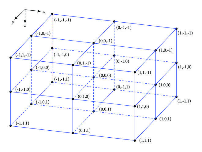
The phrase "discretized three-dimensional" gives us a clue about why it uses a "27-point stencil at each grid point in the 3D domain."

If you look at the image, starting from the point (0,0,0), you see 26 surrounding points plus the center, making 27 points. This means that one row in the matrix can have up to 27 non-zero elements, with each element representing a point in 3D space. However, the boundary points might have 7 to 18 non-zero elements, and I'm not entirely sure why—I'll leave that mystery for now. Shouldn't it be 8? I wish someone enlightens me on this.

The problem assumes that the values inside the solution vector are 1.0, but this should not be exploited. Also, while properties like symmetry, positive definiteness, and non-singularity are used in the computations, don't hardcode any data structures based on these assumptions.

This should be enough to start working on the program.

Computations

Looking at the list of files in the HPCG source code, we can identify the main computations required for the benchmark. Some of these are key operations to optimize.

From here on, I'll focus on the actual computations, not their mathematical implications.

• CG: Conjugate Gradient. It consists of other basic computations below.
• DotProduct: Dot product of two vectors.
• MG: Multigrid method. It returns approximated $x$. I'll explain it later. It includes SPMV and SYMGS inside it.
• SpMV: Sparse Matrix-Vector Multiplication. It's similar to a regular matrix-vector multiplication, but with sparse matrices.
• SYMGS: Symmetric Gauss-Seidel. It also returns some relevant $x$. It'll also be explained.
• WAXPBY: Weighted AXPBY operation. $y = \alpha x + \beta y$

Multigrid (MG)

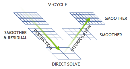
Multigrid approximates the solution of the linear system using "coarse" matrices. A "fine" matrix is the original high-resolution one, while a "coarse" matrix has lower resolution, derived from the finer one. It's like solving an easier, lower-resolution version of the problem and using that solution to help solve the original one. Here's what happens in the MG operation:

1. Pre-smoothing: Using SYMGS, it smooths out the oscillations in the error. That's why it's called "smoothing." Regarding SYMGS, we will see it later.
2. Restriction: It sets the "coarse" residual ($r$) (or, we can call it downsampling). It's a simple operation that's done only in a line a code.
3. Recursive MG: Do the same MG operation for the coarser matrix.
4. Prolongation: It's the oposite of the Restriction. It sets the "fine" residual ($r$) from the "coarse" residual. It's also a simple operation that's done only in a line a code.
5. Post-smoothing: Again, using SYMGS, it smooths out the oscillations in the error.

Restriction and Prolongation doesn't add much to the total time, but it's important for understanding how MG works. (Yes, they are also in the scope of optimization, as it's used inside the MG operation.)

SYMGS (Symmetric Gauss-Seidel)

This iteratively refines the approximate solution $x$. It consists of "Forward" and "Backward" sweeps, which basically do the same thing. The arithmetic operations are straightforward, but what's important is the pattern in which it accesses data.

• It iterates through the rows in $A$ (let's say the current row is $i$).
• It accesses the value of $r$ corresponding to the current row $i$.
• Inside the row, 1) it takes the diagonal value ($A[i][i]$) and 2) iterates through the non-zero values in the row.
• And set the value of $x$ corresponding to the current row $i$.

Moreover, we can find that though it does simple operations, it should be done in sequence.

  for (local_int_t i=0; i< nrow; i++) {
    const double * const currentValues = A.matrixValues[i];
    const local_int_t * const currentColIndices = A.mtxIndL[i];
    const int currentNumberOfNonzeros = A.nonzerosInRow[i];
    const double  currentDiagonal = matrixDiagonal[i][0];
    double sum = rv[i];

    for (int j=0; j< currentNumberOfNonzeros; j++) {
      local_int_t curCol = currentColIndices[j];
      sum -= currentValues[j] * xv[curCol];
    }
    sum += xv[i]*currentDiagonal;
    xv[i] = sum/currentDiagonal;
  }

To update $x[i]$, values from other parts of $x$ are required. This interdependency means that, strictly speaking, the computation isn't parallelizable. However, the algorithm allows for some relaxation. Since this is an iterative method, each iteration doesn't need to be perfectly precise; the goal is simply to ensure convergence over multiple iterations. Therefore, instead of preserving strict dependencies, we can relax them slightly to enable parallelization. This relaxation trades off some precision in individual iterations for overall efficiency, ultimately still achieving convergence.

SpMV

Sparse Matrix-Vector Multiplication does't need much explanation. Just remember that the matrix is sparse, making this operation memory-bound rather than compute-bound. SpMV and SYMGS are the most time-consuming parts of the benchmark and are key targets for optimization.

Optimizations

Main Focus

As we saw in SYMGS and SpMV, the main performance bottleneck is memory access. Unlike LINPACK, achieving the theoretical peak FLOPS performance in HPCG is challenging due to its memory-bound nature. Even highly optimized systems often fall short of the theoretical maximum. The key is to optimize data access patterns. Also, further parallelization should be implemented for SYMGS. Multicoloring is for this. They use "JPL" coloring for rocHPCG, and I guess it means Jones-Plassmann-Luby.

Permitted

• Memory Allocations: The You can optimize the memory access patterns to improve cache utilization
• Sparse Matrix Format: The default is Compressed Sparse Row (CSR), but other formats like ELLPACK can be used. The official documentation encourages ELLPACK to minimize pointer references and cache misses.
• Parallelization: OpenMP and MPI are enabled by default but the code isn't fully optimized.
• Multi-coloring can be used to enable further parallelization, as suggested in the official documentation.
• You can also use SIMD or other parallelization techniques.
• Using Libraries: BLAS, MKL, or other libraries can be used to optimize specific computations.
• Compiler Optimizations: Utilize a good compiler, -O3 optimization, and other relevant flags.

Not Permitted

• Precision Changes: Don't use quantization or change data types.
• Algorithmic Changes: The same mathematical algorithm must be used, with no changes, only optimizations.
• Hardcoding / Exploits: Avoid exploiting known matrix characteristics like symmetry with storing only the half of the values. Assume random values.

Conclusion

I'll begin with the reference implementation and gradually work on optimizing it step by step. In the next article, I'll start with a basic analysis of the reference implementation and then dive into the optimization process.

References

• HPCG Benchmark You should start working on it by getting the reference code and running it on your system.

• rocHPCG Practically, they've done almost any optimizations I could think of. I learned a lot from their work.

• HPCG for ARM, blog post 1 and blog post 2 It explains how they optimized the HPCG benchmark for ARM architecture. It's a good reference for getting hints on how to optimize the benchmark.

• Performance modeling of the HPCG benchmark It gives the insight on how the performance of the benchmark can be modeled, that is, what affects the performance of the benchmark most.